Beginning programmers are taught to learn how to write “Hello World” as their first programming exercise. For khipu scholars, who are researching khipus statistically, Benford’s Law is their “Hello World.” Benford’s law, simply put, says that the first digits of numbers used to measure human activity tend to have a higher probability that they are 1. For example, 10,000, 1,000, etc. We can use Benford’s law to predict which khipu are of an “accounting nature” - ie. khipu that have sums and accounts of things.
The first digit (or leading digit) of a number is the leftmost digit (e.g. the first digit of 567 is 5). The first digit of a number can only be 1, 2, 3, 4, 5, 6, 7, 8, and 9 since we do not usually write a number such as 567 as 0567. Some fraudsters may think that the first digits in numbers in financial documents appear with equal frequency (i.e. each digit appears about 11% of the time). In fact, this is not the case. It was discovered by Simon Newcomb in 1881 and rediscovered by physicist Frank Benford in 1938 that the first digits in many data sets occur according to the probability distribution indicated in Figure 1 below:
The above probability distribution is now known as the Benford’s law. It is a powerful and yet relatively simple tool for detecting financial and accounting frauds. For example, according to the Benford’s law, about 30% of numbers in legitimate data have 1 as a first digit. Fraudsters who do not know this will tend to have much fewer ones as first digits in their faked data.
Data for which the Benford’s law is applicable are data that tend to distribute across multiple orders of magnitude. Examples include income data of a large population, census data such as populations of cities and counties. In addition to demographic data and scientific data, the Benford’s law is also applicable to many types of financial data, including income tax data, stock exchange data, corporate disbursement and sales data. The author of I’ve Got Your Number How a Mathematical Phenomenon can help CPAs Uncover Fraud and other Irregularities., Mark Nigrini, also discussed data analysis methods (based on the Benford’s law) that are used in forensic accounting and auditing.
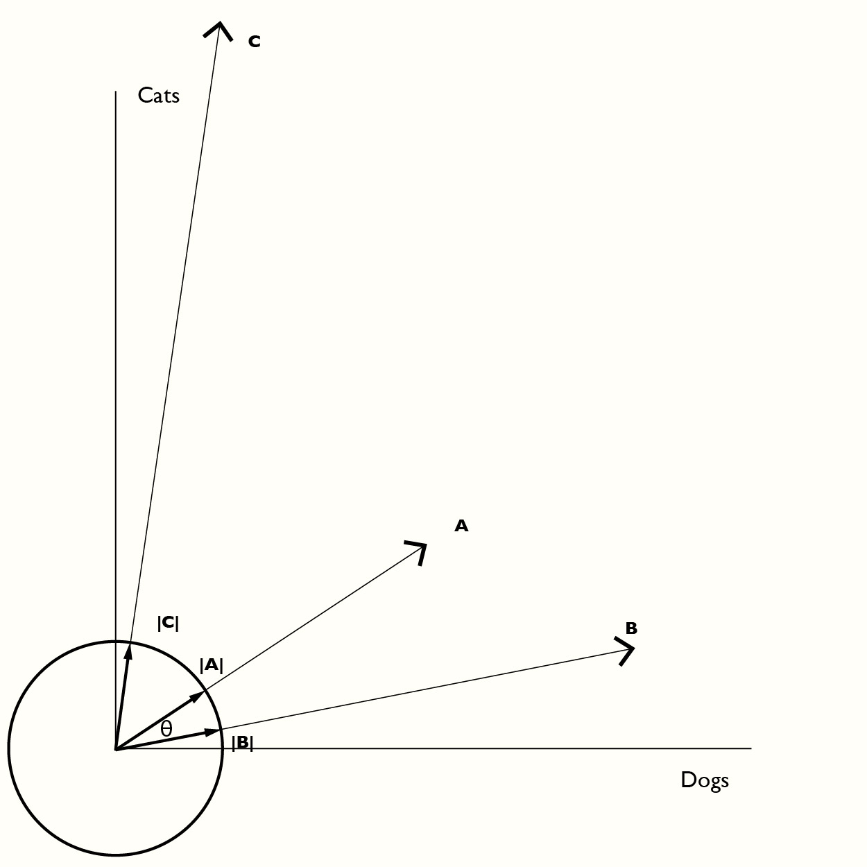
Using the distribution of “first digits” in a cord (the value of the first knot) we can use a simple cosine distance similarity metric of Benford’s distribution and cord distribution. Cosine distance similarity is a simple concept that is used a lot in this study … If you’re unfamiliar here’s an intuitive explanation.
Suppose we want to see how close two sets of numbers are to each other. For example house A has 3 dogs and 2 cats, house B has 5 dogs and 1 cat and house C has 1 dog and 7 cats. We can represent each of these as a vector:
A = [3,2] B = [5,1] C = [1,7]
Each of these vectors can be “normalized” to a unit vector (a vector of length 1) by dividing by the vector length. Then you can take advantage of math. A vector dot-product of two vectors measures the angle between those two vectors. If we want to know if A is closer to B or C we take A . B and A . C and see which has the smallest angle between them. The dot -product generates the cosine of the angle, which is why this technique is known as the cosine distance metric.
We can do the same for khipus by creating a vector of first digit counts, for a given khipu and then dot producting it with the Benford probabilities above.
f(angle_theta) = first_digit_probability . given_khipu_digit_distribution. If the angle theta is 0, the vectors lie on top of each other (an exact match) so cos(theta) = 1, with no match = 0.
Another approach to understanding which khipus are accounting in nature, and which aren’t is to sum up cord values and see if that sum occurs elsewhere on another cord in the khipu. Dr. Urton, shows an example of this kind, khipu KH0263, in his youtube video on accounting khipu. Here I examine how many “sum matches” occur in a khipu (normalized by the number of total cords…). This gives us a secondary statistical check, in addition to Benford’s Law.
Note that the metric calculated below is not exact. Here, only two cord sums are measured. The first decoded khipu, in the 1920s by Leland Locke, had one up-cord sum for four down cord values and would not score well on this metric.
There is another metric similar to the above. Some cord groups (ie. top cords) are the sum, or approximate sum of the group adjacent (ie. on either side) of them. The khipu class tags these “sum_groups” and allows us another metric.
Code
# Initialize plotlyplotly.offline.init_notebook_mode(connected =False)# Khipu Importsimport khipu_kamayuq as kamayuq # A Khipu Maker is known (in Quechua) as a Khipu Kamayuqimport khipu_qollqa as kqall_khipus = [aKhipu for aKhipu in kamayuq.fetch_all_khipus().values()]khipu_summary_df = kq.fetch_khipu_summary()
Code
## Benford Law Similarity# Note that 0 index's are ignored, by setting first_digit_probability[0] to 0first_digit_probability = [0.0, 0.301, 0.176, 0.125, 0.097, 0.079, 0.067, 0.058, 0.051, 0.046]def benford_match(aKhipu): digit_count = [0]*10for cord in aKhipu.attached_cords(): first_digit =int(str(cord.decimal_value)[0]) digit_count[first_digit] +=1 cosine_similarity =1- scipy.spatial.distance.cosine(first_digit_probability, digit_count)return cosine_similaritykhipu_benford_match = [benford_match(aKhipu) for aKhipu in all_khipus]
We’re going to build a dataframe of benford match vs cords, and vs the number of ascher sum relationships that occur. This provides an alternative checkpoint on Benford Law matching approach, To do this we read in the previously computed Ascher Sum Relationship table, and add up all the number of ascher relationships for a given khipu
Code
fieldmarks_dir =f"{os.path.dirname(os.path.dirname(kq.qollqa_data_directory()))}/FIELDMARKS/CSV"ascher_sum_relationship_df = pd.read_csv(f"{fieldmarks_dir}/ascher_sum_relationships.csv")ascher_sums_dict = {aKhipu.name():0for aKhipu in all_khipus}for index inrange(len(ascher_sum_relationship_df)): record = ascher_sum_relationship_df.iloc[index] khipu_name = ku.strip_html(record['name']) num_ascher_sums = record['num_pendant_pendant_sum'] + record['num_pendant_pendants_color_sum'] + record['num_indexed_pendant_sum'] num_ascher_sums += record['num_subsidiary_pendant_sum'] + record['num_group_group_sum'] + record['num_group_sum_bands'] ascher_sums_dict[khipu_name] = num_ascher_sumssum_match_counts = [ascher_sums_dict[aKhipu.name()] for aKhipu in all_khipus]
Code
benford_df = pd.DataFrame({'khipu_id': [aKhipu.khipu_id for aKhipu in all_khipus],'name': [aKhipu.name() for aKhipu in all_khipus],'num_pendants': [aKhipu.num_pendant_cords() for aKhipu in all_khipus],'num_subsidiary_cords': [aKhipu.num_subsidiary_cords() for aKhipu in all_khipus],'num_total_cords': [aKhipu.num_cc_cords()for aKhipu in all_khipus],'fanout_ratio': [aKhipu.num_pendant_cords() / aKhipu.num_attached_cords() for aKhipu in all_khipus],'benford_match': khipu_benford_match,'sum_match_count': sum_match_counts})benford_df['normalized_sum_match_count'] = benford_df['sum_match_count']/benford_df['num_total_cords']benford_df = benford_df.sort_values(by='benford_match', ascending=False)display_dataframe(benford_df)
khipu_id
name
num_pendants
num_subsidiary_cords
num_total_cords
fanout_ratio
benford_match
sum_match_count
normalized_sum_match_count
252
1000269
UR053E
70
35
105
0.666667
0.992311
53
0.504762
645
6000089
UR193
99
127
226
0.438053
0.985153
87
0.384956
577
6000020
KH0058
80
98
178
0.449438
0.984313
63
0.353933
426
1000404
UR151
12
8
20
0.600000
0.978858
4
0.200000
612
6000055
QU005
57
25
82
0.695122
0.978147
6
0.073171
...
...
...
...
...
...
...
...
...
...
432
1000417
UR158
24
1
25
0.960000
0.000000
0
0.000000
159
1000445
HP026
17
0
17
1.000000
0.000000
0
0.000000
158
1000444
HP025
55
0
55
1.000000
0.000000
0
0.000000
608
6000051
QU001
33
0
33
1.000000
0.000000
0
0.000000
14
1000196
AS025
2
0
2
1.000000
0.000000
0
0.000000
651 rows × 9 columns
3. Summary Charts:
Code
# Read in the Fieldmark and its associated dataframe and match dictionaryfrom fieldmark_khipu_summary import Fieldmark_Benford_MatchaFieldmark = Fieldmark_Benford_Match()fieldmark_dataframe = aFieldmark.dataframes[0].dataframeraw_match_dict = aFieldmark.raw_match_dict()
# Plot Significant khipusignificant_khipus = [aKhipuName for aKhipuName in matching_khipus if raw_match_dict[aKhipuName] >0.6]significant_values = [raw_match_dict[aKhipuName] for aKhipuName in significant_khipus]significant_df = pd.DataFrame(list(zip(significant_khipus, significant_values)), columns =['KhipuName', 'Value'])fig = px.bar(significant_df, x='KhipuName', y='Value', labels={"KhipuName": "Khipu Name", "Value": "Benford Match", }, title=f"Significant Khipu ({len(significant_khipus)}) for Benford Match", width=944, height=450).update_layout(showlegend=True).show()
4. Significance Criteria:
What is deemed “significant”
Code
hist_data = [khipu_benford_match]group_labels = ['benford_match']colors = ['#835AF1'](ff.create_distplot(hist_data, group_labels, bin_size=.01, show_rug=False,show_curve=True) .update_layout(title_text='Distribution Plot of Khipu -> Benford Matches', # title of plot xaxis_title_text='Benford Match Value (cosine_similarity)', yaxis_title_text='Percentage of Khipus', # yaxis label bargap=0.05, # gap between bars of adjacent location coordinates#bargroupgap=0.1 # gap between bars of the same location coordinates ) .show())
Here’s a clear statistical/graphical narrative as to which khipus are “accounting” in nature (from a little above .6 to 1.0!), somewhat accounting in nature (.4 to .6), and possibly narrative in nature (< 0.4). How many khipus in each category?
Let’s do a scatter plot of Benford Matching vs (normalized) cords whose values match another set of cords (ie. one of the Ascher X-ray Sum Relationships). The grouping of accounting khipus is revealed even more clearly.
Code
fig = px.scatter(benford_df, x="benford_match", y="normalized_sum_match_count", log_y=True, size="num_total_cords", color="num_total_cords", labels={"benford_match": "#Benford Match", "normalized_sum_match_count": "#Number of Matching Cord Sums (Normalized by # Total Cords)"}, hover_data=['name'], title="<b>Benford Match vs Normalized Ascher Sum Relationship Counts</b> - <i>Hover Over Circles to View Khipu Info</i>", width=944, height=944);fig.update_layout(showlegend=True).show()
Again, we see the lumpiness and confirmation of the “accounting khipus” whose Benford match is > 0.6 or so….But we ALSO see high evidence of summation relationships in low benford match khipu which have a large number of cords. This is not a good graphic for the argument that khipus are written speech!
Sanity Check - Marcia Ascher’s “Mathematical” Khipus versus their Corresponding Benford Match
As another checkpoint on Benford Law matching approach, let’s review the reverse - khipus that Marcia Ascher’s annotated with mathematical relationships and compare them with their corresponding Benford match distributions
Code
# These are the khipus that Marcia Ascher annotated as having interesting mathematical relationshipsascher_mathy_khipus = ['AS010', 'AS020', 'AS026B', 'AS029', 'AS038', 'AS041', 'AS048', 'AS066', 'AS068', 'AS079', 'AS080', 'AS082', 'AS092', 'AS115', 'AS128', 'AS129', 'AS164', 'AS168', 'AS192', 'AS193', 'AS197', 'AS198', 'AS199', 'AS201', 'AS206', 'AS207A', 'AS208', 'AS209', 'AS210', 'AS211', 'AS212', 'AS213', 'AS214', 'AS215', 'UR1034', 'UR1096', 'UR1097', 'UR1098', 'UR1100', 'UR1103', 'UR1104', 'UR1114', 'UR1116', 'UR1117', 'UR1120', 'UR1126', 'UR1131', 'UR1135', 'UR1136', 'UR1138', 'UR1140', 'UR1141', 'UR1143', 'UR1145', 'UR1148', 'UR1149', 'UR1151', 'UR1152', 'UR1163', 'UR1175', 'UR1180']ascher_khipu_benford_match = [benford_match(aKhipu) for aKhipu in all_khipus if aKhipu.name() in ascher_mathy_khipus]def is_an_ascher_khipu(aKhipu):returnTrueifstr(aKhipu.original_name)[0:2] =="AS"or aKhipu.name()[0:2] =="AS"elseFalseascher_khipus = [aKhipu for aKhipu in all_khipus if is_an_ascher_khipu(aKhipu)]percent_mathy_khipus =100.0*float(len(ascher_mathy_khipus))/float(len(ascher_khipus))percent_string ="{:4.1f}".format(percent_mathy_khipus)hist_data = [ascher_khipu_benford_match]group_labels = ['benford_match']colors = ['#835AF1'](ff.create_distplot(hist_data, group_labels, bin_size=.01, show_rug=False,show_curve=True) .update_layout(title_text='<b>Benford Match for Ascher Khipus with Mathematical Relationships</b> - <i>Hover Over Circles to View Khipu Info</i>', # title of plot xaxis_title_text='Benford Match Value (cosine_similarity)', yaxis_title_text='Percentage of Khipus', # yaxis label bargap=0.05, # gap between bars of adjacent location coordinates#bargroupgap=0.1 # gap between bars of the same location coordinates ) .show())print (f"Percent of ascher khipus having mathematical relationships ({len(ascher_mathy_khipus)} out of {len(ascher_khipus)}) is {percent_string}%")
Percent of ascher khipus having mathematical relationships (61 out of 144) is 42.4%
We see that all of Ascher’s khipus that Marcia Ascher analyzed have a Benford match over 0.4. This is no surprise, but it’s a good confirmation that the technique makes sense.
Benford Match vs Fanout Ratio (Primaries vs Subsidiaries)
Let’s conclude this section with an interesting “triangular” graph - Benford match vs Fanout Ratio (the ratio of Pendant cords vs Subsidiary cords)
If khipus are indeed linguistic, we would expect their cords to take on one of two possible linguistic structures:
Linear/Serial Structure: One possibility is that language is encoded serially with each cord expressing a morpheme or word. The Zipf’s Law study below explores this possibility.
Tree Structure: The other possibility is that language is expressed in a tree fashion, using primaries and subsidiaries, like the sentence diagrams you used to do in grade school. The above Benford’s law Fan-out study suggests that encoding in a tree fashion is highly unlikely.
The only significant khipu to appear in the lower left triangle is KH0329. However, an examination of the Ascher sum relationships for this khipu show it to have significant arithmetic relationships.
7. Zipf’s Law
Another approach to understanding if khipus are linguistic in nature, is an examination of their various distributions of color, cord-value, etc., according to Zipf’s law. Zipf’s Law, as a linguistic measure has been extensively studied, and it’s general conclusions apply to all forms of human language.
Zipf’s Law, like Benford’s Law is a similar power curve, although it is different in distribution than Benford’s Law. A study of khipus, using Zipf’s Law, once again, diminishes the argument that khipus are linguistic in nature.
8. Conclusion
There are many statistical “leading indicators” that imply that khipus are most likely not linguistic.
Application of Benford’s Law, indicates that the majority of found khipus have numbers that closely fit with distributions of numbers used in human “accounts” such as taxes, inventories, census data, etc.
The significant presence of Ascher Sum relationships such as pendant sums of other pendants, or group sums of other groups, in low Benford match khipus, implies, fairly strongly, that khipus are not a medium of literature or writing (in the western sense of the word), but rather an accounting structure of some sort.
Application of Zipf’s Law, adds considerable statistical weight to the argument that khipus do not have a “natural language vocabulary” whether color, cord-value, or overall structure. These three possible linguistic communication media, all fail to follow a classic Zipfian natual language distribution.
Only cord-values obey the Zipfian natural language distribution of hapax legomena - the 40-60% of vocabulary that is only used once. Cord colors fail miserably on this measure.
It could be argued that the small amount of data we have in khipus prevents us from achieving a reasonable Zipfian fit for documents, cord colors, and cord values. That would explain the drop off in low-ranking/ high-frequency words, but not the erratic fit of high-ranking/low-frequency words. Similarly, we know that cord-colors are off the chart abnormal for zipfian distribution - ie. their low percentage of hapax legomena (perhaps caused by a limited color palette or a limited sample size). The only thing that is Zipfian normal is cord-values although that too is a poor fit.