Hierarchical Clustering

---

1. Hierarchical Clustering

Sorting Khipus - What Constitutes “Similarity” and “Difference”?

As a useful first step, it will help to have the ability to sort khipus not just by meta-features like benford_match, but also by other forms of similarity.

One of my favorite similarity techniques is the text-clustering approaches of NLP. A driving need in NLP is to sort topics into various categories; for example, is this a news document or fiction. So how do we text mine khipus? A simple solution is to convert the khipu to words. Each Python Khipu class object (Knot, Cord, Cluster, etc.) is given a “writer” function that documents itself as text. Below is the “document” for a simple 3 cord khipu - AS055. It’s a pretty sparse and simple description. We’ll go about making this more sophisticated as the project becomes more developed. The point is that we now have a set of words that roughly describe a khipu with categorical words such as U_knot_twist, or single_knot and numerical words such as 1421_decimal_value for the cord value. Now we use that set of words as the input to NLP algorithms.

Code

# Initialize plotly
plotly.offline.init_notebook_mode(connected = False);

# Khipu Imports
import khipu_kamayuq as kamayuq  # A Khipu Maker is known (in Quechua) as a Khipu Kamayuq
import khipu_qollqa as kq
all_khipus = [aKhipu for aKhipu in kamayuq.fetch_all_khipus().values()]
khipu_summary_df = kq.fetch_khipu_summary()

khipu_docstrings_df = kq.fetch_khipu_docstrings()
khipu_names = list(khipu_docstrings_df.kfg_name.values)
khipu_documents_orig = list(khipu_docstrings_df.document.values)

# To assist clustering Ascher khipus, where many khipu metrics such as cord attachment, twist, etc are unknown, 
# We can impute values for attachment, cord twist and knot twist
khipu_documents = [aDocument.replace("Unknown_attachment_type", "Recto_attachment_type").replace("U_twist", "S_twist").replace("U_knot_twist", "S_knot_twist") for aDocument in khipu_documents_orig]

Code

text_rep = khipu_docstrings_df[khipu_docstrings_df.kfg_name=="AS055"].document.values[0]
print(ku.multiline(text_rep))

 primary_cord_start YB cord_cluster_start 1_cluster_level 3_cc_cords cord_start 
 U_attachment_type U_twist 1_cord_level 1_cord_ordinal 1421_decimal_value 
 1_cluster_ordinal KB knot_cluster_start single_knot U_knot_twist ʘ_knot_value 
 knot_cluster_end knot_cluster_start single_knot U_knot_twist o_knot_value 
 single_knot U_knot_twist o_knot_value single_knot U_knot_twist o_knot_value 
 single_knot U_knot_twist o_knot_value knot_cluster_end knot_cluster_start 
 single_knot U_knot_twist •_knot_value single_knot U_knot_twist •_knot_value 
 knot_cluster_end knot_cluster_start figure_eight_knot U_knot_twist ※_knot_value 
 knot_cluster_end cord_end cord_start U_attachment_type U_twist 1_cord_level 
 2_cord_ordinal 2427_decimal_value 2_cluster_ordinal YB knot_cluster_start 
 single_knot U_knot_twist ʘ_knot_value single_knot U_knot_twist ʘ_knot_value 
 knot_cluster_end knot_cluster_start single_knot U_knot_twist o_knot_value 
 single_knot U_knot_twist o_knot_value single_knot U_knot_twist o_knot_value 
 single_knot U_knot_twist o_knot_value knot_cluster_end knot_cluster_start 
 single_knot U_knot_twist •_knot_value single_knot U_knot_twist •_knot_value 
 knot_cluster_end knot_cluster_start long_knot U_knot_twist 7_knot_value 
 knot_cluster_end cord_end cord_start U_attachment_type U_twist 1_cord_level 
 3_cord_ordinal 734_decimal_value 3_cluster_ordinal KB knot_cluster_start 
 single_knot U_knot_twist o_knot_value single_knot U_knot_twist o_knot_value 
 single_knot U_knot_twist o_knot_value single_knot U_knot_twist o_knot_value 
 single_knot U_knot_twist o_knot_value single_knot U_knot_twist o_knot_value 
 single_knot U_knot_twist o_knot_value knot_cluster_end knot_cluster_start 
 single_knot U_knot_twist •_knot_value single_knot U_knot_twist •_knot_value 
 single_knot U_knot_twist •_knot_value knot_cluster_end knot_cluster_start 
 long_knot U_knot_twist 4_knot_value knot_cluster_end cord_end cord_cluster_end 
 primary_cord_end 

Then we can pass the document to modern NLP text mining algorithms which can cluster the text by similarity along the n-dimensions of all the different words and their frequencies in each document.

The usual first step in NLP document analysis is to build a term-frequency, inverse-document-frequency matrix.

Tf-Idf matrices for NLP have a long history. An explanation:

Term Frequency, Inverse Document Frequency and Tf°Idf

As part of training our machine model, we want to give it information about how words are distributed across our set of data. This is commonly done using Term Frequency/Inverse Document Frequency techniques.

The first step, then, is to calculate the term frequency (Tf), the inverse document frequency (Idf), and their product (Tf°Idf) Apologies: There’s an occasional Google Chrome bug with latex/equation rendering - see equations in Safari if you want to understand them

(Tf): TERM FREQUENCY - How probable is that this particular word appears in a SINGLE document.

\(Tf(\omega) = \left( \frac{ \# occurrences\ of\ \omega\ in\ document}{\# words\ in\ document} \right)\)

(Idf): INVERSE DOCUMENT FREQUENCY - How common or rare a word is across ALL documents. If it’s a common word across all documents, it’s regarded as a non-differentiating word, and we want to weight it lower.

Alternatively, it can be thought of as the specificity of a term - quantified as an inverse function of the number of documents in which it occurs. The most common function used is log(natural) of the number of docs divided by the number of docs in which this term appears.

\(Idf(\omega) = ln \left( \frac{ \# docs}{\# docs.containing(\omega) } \right)\)

(Tf°Idf):TERM SPECIFICITY Tf°Idf, the product of Tf and Idf, is used to weight words according to how “important” they are to the machine learning algorithm ☺. The higher the TF°IDF score (weight), the rarer the term and vice versa. The intuition for this measure is this:

If a word appears frequently in a document, then it should be important and we should give that word a high score. But if a word appears in too many other documents, it’s probably not a unique identifier, therefore we should assign a lower score to that word.

Tf°idf is one of the most popular term-weighting schemes today. Over 80% of text-based recommender systems, including Google’s search engine, use Tf°Idf. Introduced, as “term specificity” by Karen Spärck Jones in a 1972 paper, it has worked well as a heuristic. However, its theoretical foundations have been troublesome for at least three decades afterward, with many researchers trying to find information theoretic justifications for it.

Ashok Khosla - Detecting Deceptive Hotel Reviews

Code

# Calculate TF-IDF Matrix

def simple_tokenizer(text):
    # first tokenize by sentence, then by word to ensure that punctuation is caught as it's own token
    tokens = [word.lower() for word in nltk.word_tokenize(text)]
    return tokens

tfidf_vectorizer = TfidfVectorizer(max_df=.9, max_features=200000,
                                   min_df=.1, stop_words=None,
                                   use_idf=True, tokenizer=simple_tokenizer, ngram_range=(1,10))

tfidf_matrix = tfidf_vectorizer.fit_transform(khipu_documents)

terms = tfidf_vectorizer.get_feature_names()
cosine_distance = 1 - cosine_similarity(tfidf_matrix)

2. Search Criteria:

Hierarchical clustering, uses “cosine similarity” (i.e. how close together are two normalized vectors in an n-dimensional bag-of-words frequency matrix) to group together and cluster documents. In my experience, it generally performs better than Kmeans or Principal Component Analysis. Although I prefer the R graphics package for clustering, Python provides graphics adequate for the job at hand:

Code

Z = ward(cosine_distance) #define the linkage_matrix using ward clustering pre-computed distances

3. Significance Criteria:

What exactly are we measuring when we cluster? That’s a difficult question to answer. How good is the clustering? Again a difficult question to answer. Later, in phase 3, we can see if we can determine useful eigenvectors of a khipu (something like Fieldmarks, but hopefully more comprehensive!), the mathematical equivalent of archetypal khipus that are the basis of all khipus. Until then, a simple plot of our hierarchical clustering with respect to benford_match and color shows that hierarchical clustering is occuring i.e. lots of clusters of little hills, but not as we expect, i.e. montonically decreasing.

The khipus simply defy simple explanation. As Piet Hein says:

Problems worthy
Of attack,
Prove their worth,
By hitting back.

4. Summary Charts:

Code

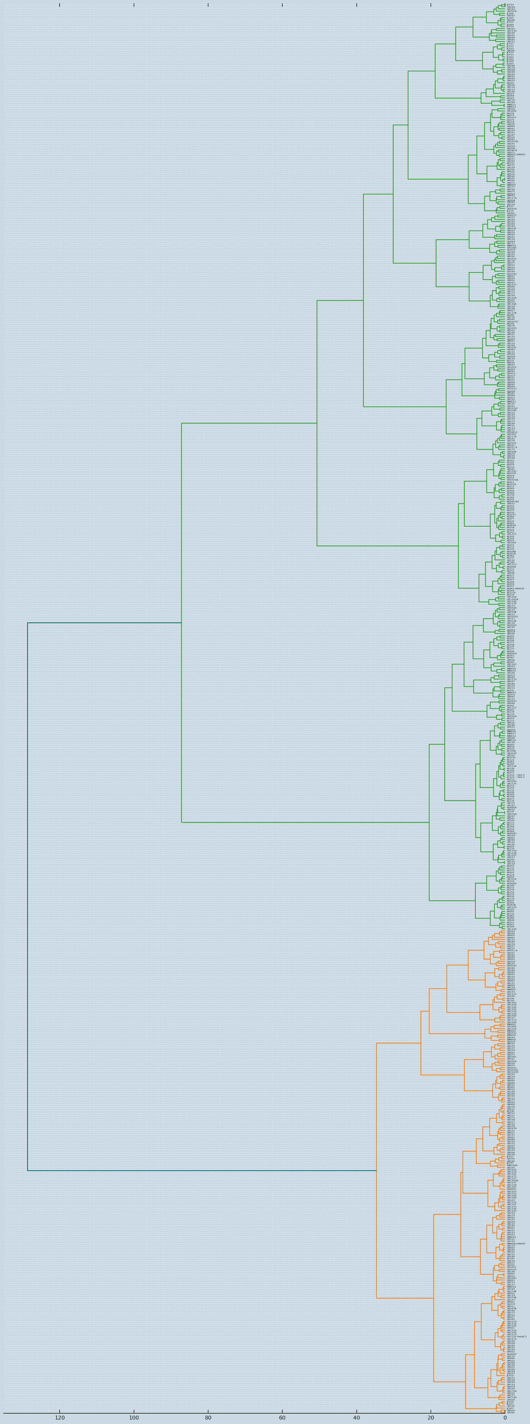
# Initialize plotly
plotly.offline.init_notebook_mode(connected = False);

fig, ax = plt.subplots(figsize=(15, 40)) # set size
ax = dendrogram(Z, orientation="left", labels=khipu_names);

plt.tick_params(\
    axis= 'x',          # changes apply to the x-axis
    which='both',       # both major and minor ticks are affected
    bottom='off',       # ticks along the bottom edge are off
    top='off',          # ticks along the top edge are off
    labelbottom='off')

plt.tight_layout() #show plot with tight layout

#uncomment below to save figure
plt.savefig('./images/khipu_clusters.png', dpi=200) #save figure as ward_clusters

# Clustered 
sorted_by_similarity = ax['ivl']
#print(sorted_by_similarity)

Sanity Check - Calendar Khipus

Again, you can examine the results visually using the Khipu Fieldmark Browser. As a sample of how well this hierarchical clustering occurs, let’s look at how close UR006, UR009, UR021, and UR1084/AS084 cluster. These 4 khipus are all considered to be “astronomical” or calendar type khipu, based on their cluster frequencies and cords per cluster. You can see that the clustering algorithm correctly places UR006, UR009 and UR021 close together, but it places UR1084 much farther away. Why? I’ll have to analyze Juliana Martin’s work on UR1084 more in phase 2 or 3.

Code

calendar_khipus = ['UR021', 'UR006', 'UR009', 'UR1084']
for i, aKhipu in enumerate(calendar_khipus):
    previous_khipu_name = calendar_khipus[i-1] if i > 0 else calendar_khipus[0]
    cur_khipu_name = calendar_khipus[i]
    previous_khipu_index = sorted_by_similarity.index(previous_khipu_name)
    cur_khipu_index = sorted_by_similarity.index(cur_khipu_name)
    delta_previous = abs(cur_khipu_index - previous_khipu_index)
    print(f"{aKhipu} is at position: {cur_khipu_index} - {delta_previous} away from previous khipu")

UR021 is at position: 494 - 0 away from previous khipu
UR006 is at position: 475 - 19 away from previous khipu
UR009 is at position: 473 - 2 away from previous khipu
UR1084 is at position: 178 - 295 away from previous khipu

5. Conclusion

There are many types of computer-generated khipu “typologies”. Most rely on on abstractions of the khipu such as provenance, or number of cords per cluster - not unlike our fieldmarks. This typology/sorting rely’s on a textual description of the khipu itself. As seen visually, using the Khipu Fieldmark Browser the approach appears to have a measure of the success. That it seems to group fieldmarks together, as well as calendars, shows one benefit of this micro-level approach to khipu analysis.